Whole document tree
Chapter 13. Solver
13.1. Solver
With Gnumeric Solver you can solve linear programs.
13.1.1. Introduction to Linear Programming
A linear program (LP) is a problem that can be expressed as linear functions. As you probably already know, a linear function is the one whose graph is always a straight line. Thus each variable of it appears in a separate term with its coefficient. There must be no products or quotients of these variables. In addition, the exponent of each term must be one. No logarithmic, exponential, trigonometric terms are allowed. Especialy note that functions like ABS, IF, MAX, and MIN are not linear. Here are a few examples of linear functions:
    3x + y - 5z
    -3.23x + 0.33y
    -0.3x + 4y - 2z + 1.2m
The linear problem has a so called objective function which is to be minimized or maximized and constraints. The objective function is the one whose value we would like to optimize. Typically, this function could determine the profit generated by the expected sales of the given model (maximization problem), or, the cost of the production in the given environment (minimization problem). Anyway, on purely mathematical point of view, we could examine the following objective function:
Maximize 2x + 3y - z
In linear programming the variables of this functions are not allowed to take any values (otherwise the maximum of any objective function would be infinity). The problem also has constraints. The constraints are a set of linear functions and a set of their right hand side values (RHS). For example, for the previously defined objective function we have the following constraints:
    x + y <= 5           (#1)
    3x - y + z <= 9      (#2)
    x + y >= 1           (#3)
    x + y + z = 4        (#4)
    x, y, z >= 0         (non-negativity assumption)
This constraint set consists of three unequality constraints (#1-#3) and one equality constraint (#4). Their RHS values are 5, 9, 1, and 4. In addition, we also have the non-negativity assumption. That is, all the variables (x, y, and z) have to take only positive numbers. The idea is to find the optimal values for the variables (x, y, and z) but also to satisfy all the given constraints.
13.1.2. Spreadsheet Modeling
To solve optimization problems with Gnumeric you have to type in the problem into a sheet. A recomended way to start with is to allocate a separate column in the spreadsheet for each decision variable (in the previous example the x, y, and z) and a separate row for each constraint (the constraints #1-#4). The coefficients of these variables should be placed into the cells corresponding to the allocated row and the column. It is also recomended that you label the rows and the columns to make the sheet much more readable. The sheet for our maximization problem would look like this:
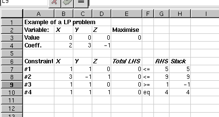
As you can see, we have put the model variables into cells B3:D3. They are currently all zeros. The cell E3 contains the objective function definition. The easiest way to define it is to use SUMPRODUCT build-in function. Thus in our model, we have the formula `=SUMPRODUCT(B3:D3,B4:D4)' in E3.
The constraints are defined in rows seven to ten. Since the coefficients of these functions are in columns B, C and D we will get the total sum of each of the constraint using the formula `SUMPRODUCT(B$3:D$3,Bn:Dn)' where n is the row number of the constraint. For example, in E7 we have `=SUMPRODUCT(B$3:D$3,B7:D7)', in E8 `=SUMPRODUCT(B$3:D$3,B8:D8)' and so on. The right hand side (RHS) values of the constraints are typed into cells G7:G10.
Now it is time to select `Solver...' from the `Tools' menu. After you have done it, the following dialog will appear:
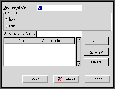
Since we have the objective function in E3 type this into the `Set Target Cell:' entry. We are about to maximize this function, thus the radiobutton `Max' should be pressed on. By default, the problem is assumed to be maximization problem. The input variables (x, y, and z) were in cells B3:D3 so type the cell range into the `By Changing Cells:' entry. Now we can add the constraints. Click Add button and the following dialog will appear.
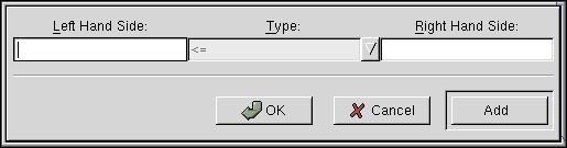
Now type in the constraints (#1-#4) one by one. The constraint dialog has three entry boxes. Put a cell name of the total left hand side (LHS) cell into the `Left Hand Side:' entry box. In our example, this would be E7 for the constraint #1, E8 for constraint #2, and so on. The combo entry in the middle defines the type of the constraint. It can be `<=', `=', `>=', or `Int'. We will explain the `Int' constraints later. In this example, you should select `<=' for constraints #1-#2, `>=' for #3, and `=' for constraint #4. The last entry on the right takes the right hand side values of the constraints. For constraints #1-#4 they should be 5, 9, 1, and 4 in this order. After typing each constraint press Add button if you still want to add more constraints after this one, or, press Ok button after typing the last constraint. When you have typed in all the constraints, the Solver dialog should look like this:
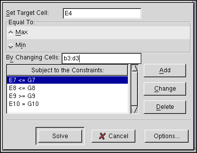
The order of the constraints does not matter. If you want to change or delete a constraint click it and then press `Change' or `Delete' button. If everything looks ok, we should check the current settings of the Solver options by pressing the Options... button. Since the problem is a linear problem the checkbutton called `Assume linear model' should be checked on. In addition, since we want the variables to be positive in our problem setting, in this case, we should also have the `Assume non-negative' button checked on. Click OK when done. Now it's time to press the Solve button. If everything went ok, the following window will appear:
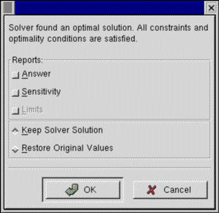
If you look the sheet, you will notice that X and Z are set to zero and Y is set to four. It means that in the optimal solution Y=4 and X=Z=0.
13.1.3. Integer Programming
You can use the Solver tool also for integer programming (IP) and more generally mixed integer programming. In integer programming some of the decision variables are required to take on integer values. To do so, just add a constraint whose type is `Int'.